The Finite Elements Method convergence survival guide

Ok, people, let’s face it. Many of us had no idea about the maths behind Finite Elements Method (FEM) simulations when we initially started using them. And most of us have felt that horrible feeling when we repeatedly saw the message ‘No convergence’ instead of a nice output. What is horrible about it is that, unless you or your group develops the software, you probably have no idea where to start looking for fixing the problem.

I heard from a lot of people in my field (electronics) that they have felt discouraged with FEM and did not even want to touch it. But I’m here to tell you that there is hope! I decided to write this guide after almost 10 years of using this type of software (on and off), first for nanoelectonics and then for semiconducting quantum technologies. It might be that the issue is actually more important in the latter, because of the differences in magnitude (or the scale of things) between classical and quantum effects (yes, not everything is quantum in quantum TCAD). But this is a user’s and not developer’s guide, so I will also keep it math-and code-free.

Where does the convergence problem come from?

So, before going through the solution proposals let’s get an intuitive idea about the convergence problem. When you press run, your simulator is numerically trying to solve a set of equations. From the very basic maths knowledge we know that there are cases when we cannot solve one equation with a specific method, like for example derivatives through discontinuities. A numerical method uses a lot of approximations to go around this problem, but sadly it also has its limitations.

Also, unless you are using some very specialized feature, the simulator will be using linear algebra to solve a given task. But what happens when your system is non-linear? Unlikely for spatial solutions in electrostatics, but for time-dependent simulations it can very well be non-linear from one solution to the next. Any BIG abrupt change from one numerical value to another can make the simulation stop with this horrible message.

What’s worse, even if the model runs and you have a solution, the solution might not be correct. Relax, though, because that rarely happens, and if it does it is usually accompanied by unending running time, large errors and difficulty in achieving convergence, if ever. Personally, I have yet to see such a situation in my simulations since in the end the results are compared either to analytical equations or experiments.

Why interfaces are prone

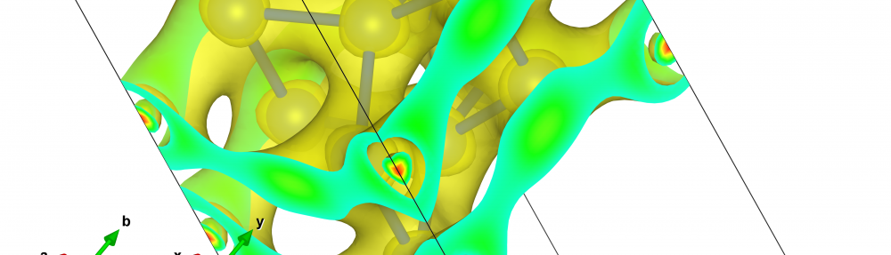
Most TCAD manuals focus their convergence advice on interfaces. The reason that they insist is because this is the location where the variables of the models, and sometimes even the models themselves, change. This change needs a fine meshing in order to capture the correct change in the various functions to be solved (electric field, potential energies, densities etc.).

Look for example in the figure below the output from a model with a failed convergence. I am plotting the electron temperature only at the material on the right, while the dark red and pink colors signify a different material. At two mesh locations on the interface, the value of temperature is really high. This of course is just a numerical artefact due to the failed convergence.

Picture of interface in an electronic device after failed convergence. Electrons getting really ‘hot’ at this location.

Sadly, we get no information on how to solve the problem with plots like this. You can try using a progressively finer mesh, and this might do the trick. Unfortunately, there are cases where this is not enough.

This is the case of ‘singularities’, or locations where infinitely high values appear. (Note: You can find a nice plot of this problem and more ideas here). Singularities are the easiest to solve, but they are not easy to find because we (at least me) are usually looking elsewhere to find the problem. They can arise in electronics, especially when using your own 3D shapes and not a simulated fabrication flow. Placing a 3D shape and leaving just a little bit of another material in a tiny region of a few nm, next to vacuum, is a sure way of convergence problems. These may also be at the interfaces of materials, but to find them it’s best to disable all meshing information, visualize each region separately, and follow its lines to look for ‘anomalies’ in their outline.

Parameter analysis

This is probably the hardest problem to solve. The parameters that we put into the models can really take a wide range of values and be of different orders of magnitude.

Usually, professional software has default values, but they are not at all guaranteed to work for the case at hand. Instead, each model needs to be examined separately, both for its physical significance, and the values that would be more appropriate for the materials and we have. This doesn’t mean that using some crazy values will not give us the correct results. After all, it is the final device characteristics that we are interested in, and not the values of the parameters themselves. However, we want to avoid using unphysical values as this might affect other parts of the simulation, and may certainly affect convergence.

The values of the parameters that you choose can be different than what you find in the literature. This is perfectly normal. Just because these values work for some specific cases, it doesn’t mean that they will work for your model also. Also, the difference between a not so matching value from the literature and one that is close to it, might actually make the difference between having a converged and a non-converged model.

Boundary conditions

Once, while I was a PhD student, I confined my problems of convergence to someone who had more experience in systems calibration than me, and he answered ‘change the boundary conditions’. However simplistic this view, it is actually pretty accurate. Beyond the simple ‘change the applied voltage’ or ‘change from Schottky to Ohmic’, let’s imagine a few different situations:

1. You apply some voltage to the device and you cannot achieve convergence. You apply zero voltage and the model runs fine. This has happened to me a lot, and in retrospect, I have a few solutions: Start by applying a really low non-zero positive/negative voltage, like |V| = 1e-20 or 1e-10. Go higher or lower in magnitude depending on whether your model run or not respectively. When do you see it failing? Do you see any inexplicably high currents? It is possible that the parameters of the model need to be checked again, like mentioned in the previous section.
2. You run the time dependent simulations and the model runs fine, but it fails in stationary state. This can be the case if you have processes that create carriers, but not so many processes to allow the densities to ‘relax’ to an equilibrium state. This can also be avoided by changing the boundary conditions. For example, try introducing tunnelling at the interfaces, or something similar. Then the parameters will also have to be configured and probably changed so that actual convergence can be achieved in the end.
3. In both the previous cases, there is a method that is widely accepted by the FEM community, and that is ‘fake interface charges‘. This can be used when you are sure you have done all the previous correct and no further corrections to the model can save it. The idea is to create an electrostatic wall, that is ‘low enough’ (in terms of density of charges) that is practically invisible from the complete simulation, but high enough to prevent unnecessary and unphysical solutions of the equations. The fact that they are fixed, means that they are included in the overall scalar value of the potential, but not as higher order equations for the solution of i.e. the current etc.

Analytical equations

Might be painful to some, but it actually may be that solving parts of the system analytically is the way that your model can be saved. I suggest starting from simple 1D solutions of transport, before embarking on complicated 2D that take days and days to solve, because the mistake may be very simple.

Then another idea are semi-analytical solutions, where you take the output of the simulator at one mesh point and you put it into the model that interests you, and you work out the solution. I did this a lot during my PhD and it was the most structured thing I did, and also presentable to others as well.

I also suggest you take a strategic take on this, because solving parts of the system without a logic of why you are interested in that part, may result in wasting your time.

Brute forcing

If all fails, brute force! This is really the worst situations you can be is, and if you reached here, you might as well start working on another model. Sadly, I did that too in my PhD! (Literally, I had no help from no one and no software support, and I needed to finish before the end of the funding deadline).

So here is how this goes: You start by organizing your simulations very well. Any GUIs that the software has for this will be really useful if not essential. Then you take the version of the simulation model that you want (maybe also strip it down to only the necessary physical models/equations that will do the job) and start sweeping all parameters one by one within a reasonable (or crazy, you choose) range.

This is also a very consuming step, both in time and resources, but it worked for me one or two times. Hopefully, if you did the previous steps, you will not have to reach here, but this is also a ‘lazy’ way of doing things, if you skipped the others.

Convergence in quantum-classical coupled TCAD

Although I have less experience with quantum-classical software (which is normal, as they are not as many as pure classical), what I noticed early is that when including the quantum effect, convergence is much harder to achieve.

What makes this particular software a bit fussy is actually a quantum phenomenon called ‘confinement’. The mesh needs to be really fine in this case (as it is also intuitively understood) so that the electrons can move freely from one of its points to the next, without getting ‘stuck’, or localized. In fact, there is a measure of how fine it should be, and that is related to the electron wavelength. Since this is also a function of the confining potential, it can be subject to refinement.

Long story short, if you are running one of these software and you notice spatial fluctuations of the electron density with no apparent reason (no disorder potential), then I don’t think it takes more to understand that our model did not converge, or even if it did, its solution is incorrect.

A final note on this type of software is the differences in the energy scales: In quantum, all the interesting stuff happen at a very short energy range, requiring a lot of interval values. But for classical, changes happen over larger energy ranges and do not require as fine sampling intervals. While this seems like it can be solved by changing a few sweeping parameters, the truth is that also, with the quantum energy range, you need higher precision coming in from the classical part, so that the quantum part changes accordingly. This might potentially add more constrains in the convergence conditions.